Voronoi parameters#
Voronoi tessellation can be used to identify local structure by counting the number of faces of the Voronoi polyhedra of an atom. For each atom a vector \(\langle n3~n4~n5~n6\) can be calculated where \(n_3\) is the number of Voronoi faces of the associated Voronoi polyhedron with three vertices, \(n_4\) is with four vertices and so on. Each perfect crystal structure such as a signature vector, for example, bcc can be identified by \(\langle 0~6~0~8 \rangle\) and fcc can be identified using \(\langle 0~12~0~0 \rangle\). It is also a useful tool for identifying icosahedral structure which has the fingerprint \(\langle 0~0~12~0 \rangle\).
[1]:
import pyscal as pc
import pyscal.crystal_structures as pcs
import matplotlib.pyplot as plt
import numpy as np
The :mod:~pyscal.crystal_structures module is used to create different perfect crystal structures. The created atoms and simulation box is then assigned to a :class:~pyscal.core.System object. For this example, fcc, bcc, hcp and diamond structures are created.
[2]:
fcc_atoms, fcc_box = pcs.make_crystal('fcc', lattice_constant=4, repetitions=[4,4,4])
fcc = pc.System()
fcc.box = fcc_box
fcc.atoms = fcc_atoms
[3]:
bcc_atoms, bcc_box = pcs.make_crystal('bcc', lattice_constant=4, repetitions=[4,4,4])
bcc = pc.System()
bcc.box = bcc_box
bcc.atoms = bcc_atoms
[4]:
hcp_atoms, hcp_box = pcs.make_crystal('hcp', lattice_constant=4, repetitions=[4,4,4])
hcp = pc.System()
hcp.box = hcp_box
hcp.atoms = hcp_atoms
Before calculating the Voronoi polyhedron, the neighbors for each atom need to be found using Voronoi method.
[5]:
fcc.find_neighbors(method='voronoi')
bcc.find_neighbors(method='voronoi')
hcp.find_neighbors(method='voronoi')
Now, Voronoi vector can be calculated
[6]:
fcc.calculate_vorovector()
bcc.calculate_vorovector()
hcp.calculate_vorovector()
The calculated parameters for each atom can be accessed using the :attr:~pyscal.catom.Atom.vorovector attribute.
[7]:
fcc_atoms = fcc.atoms
bcc_atoms = bcc.atoms
hcp_atoms = hcp.atoms
[8]:
fcc_atoms[10].vorovector
[8]:
[0, 12, 0, 0]
As expected, fcc structure exhibits 12 faces with four vertices each. For a single atom, the difference in the Voronoi fingerprint is shown below
[9]:
fig, ax = plt.subplots()
ax.bar(np.array(range(4))-0.2, fcc_atoms[10].vorovector, width=0.2, label="fcc")
ax.bar(np.array(range(4)), bcc_atoms[10].vorovector, width=0.2, label="bcc")
ax.bar(np.array(range(4))+0.2, hcp_atoms[10].vorovector, width=0.2, label="hcp")
ax.set_xticks([1,2,3,4])
ax.set_xlim(0.5, 4.25)
ax.set_xticklabels(['$n_3$', '$n_4$', '$n_5$', '$n_6$'])
ax.set_ylabel("Number of faces")
ax.legend()
[9]:
<matplotlib.legend.Legend at 0x7f13d02b9760>
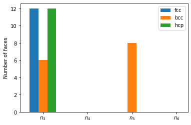
The difference in Voronoi fingerprint for bcc and the closed packed structures is clearly visible. Voronoi tessellation, however, is incapable of distinction between fcc and hcp structures.
Voronoi volume#
Voronoi volume, which is the volume of the Voronoi polyhedron is calculated when the neighbors are found. The volume can be accessed using the :attr:~pyscal.catom.Atom.volume attribute.
[10]:
fcc_atoms = fcc.atoms
[11]:
fcc_vols = [atom.volume for atom in fcc_atoms]
[12]:
np.mean(fcc_vols)
[12]:
16.0