Analyzing a lammps trajectory

In this example, a lammps trajectory in dump-text format will be read in, and Steinhardt’s parameters will be calculated.

import pyscal as pc
import os
import pyscal.traj_process as ptp
import matplotlib.pyplot as plt
import numpy as np

First, we will use the split_trajectory method from pyscal.traj_process module to help split the trajectory into individual snapshots.

trajfile = "traj.light"
files = ptp.split_trajectory(trajfile)

files contain the individual time slices from the trajectory.

len(files)

10

files[0]

'traj.light.snap.0.dat'

Now we can make a small function which reads a single configuration and calculates \(q_6\) values.

def calculate_q6(file, format="lammps-dump"):
    sys = pc.System()
    sys.read_inputfile(file, format=format)
    sys.find_neighbors(method="cutoff", cutoff=0)
    sys.calculate_q(6)
    q6 = sys.get_qvals(6)
    return q6

There are a couple of things of interest in the above function. The find_neighbors method finds the neighbors of the individual atoms. Here, an adaptive method is used, but, one can also use a fixed cutoff or Voronoi tessellation. Also only the unaveraged \(q_6\) values are calculated above. The averaged ones can be calculate using the averaged=True keyword in both calculate_q and get_qvals method. Now we can simply call the function for each file..

q6s = [calculate_q6(file) for file in files]

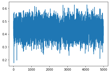
We can now visualise the calculated values

plt.plot(np.hstack(q6s))

[<matplotlib.lines.Line2D at 0x7f5e424c0f60>]

Adding a clustering condition

We will now modify the above function to also find clusters which satisfy particular \(q_6\) value. But first, for a single file.

sys = pc.System()
sys.read_inputfile(files[0])
sys.find_neighbors(method="cutoff", cutoff=0)
sys.calculate_q(6)

Now a clustering algorithm can be applied on top using the cluster_atoms method. cluster_atoms uses a condition as argument which should give a True/False value for each atom. Lets define a condition.

def condition(atom):
    return atom.get_q(6) > 0.5

The above function returns True for any atom which has a \(q_6\) value greater than 0.5 and False otherwise. Now we can call the cluster_atoms method.

sys.cluster_atoms(condition)

16

The method returns 16, which here is the size of the largest cluster of atoms which have \(q_6\) value of 0.5 or higher. If information about all clusters are required, that can also be accessed.

atoms = sys.atoms

atom.cluster gives the number of the cluster that each atom belongs to. If the value is -1, the atom does not belong to any cluster, that is, the clustering condition was not met.

clusters = [atom.cluster for atom in atoms if atom.cluster != -1]

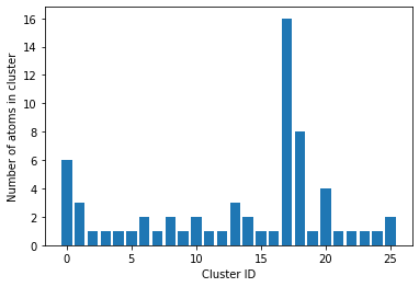
Now we can see how many unique clusters are there, and what their sizes are.

unique_clusters, counts = np.unique(clusters, return_counts=True)

counts contain all the necessary information. len(counts) will give the number of unique clusters.

plt.bar(range(len(counts)), counts)
plt.ylabel("Number of atoms in cluster")
plt.xlabel("Cluster ID")

Text(0.5, 0, 'Cluster ID')

Now we can finally put all of these together into a single function and run it over our individual time slices.

def calculate_q6_cluster(file, cutoff_q6 = 0.5, format="lammps-dump"):
    sys = pc.System()
    sys.read_inputfile(file, format=format)
    sys.find_neighbors(method="cutoff", cutoff=0)
    sys.calculate_q(6)
    def _condition(atom):
        return atom.get_q(6) > cutoff_q6
    sys.cluster_atoms(condition)
    atoms = sys.atoms
    clusters = [atom.cluster for atom in atoms if atom.cluster != -1]
    unique_clusters, counts = np.unique(clusters, return_counts=True)
    return counts

q6clusters = [calculate_q6_cluster(file) for file in files]

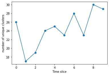
We can plot the number of clusters for each slice

plt.plot(range(len(q6clusters)), [len(x) for x in q6clusters], 'o-')
plt.xlabel("Time slice")
plt.ylabel("number of unique clusters")

Text(0, 0.5, 'number of unique clusters')

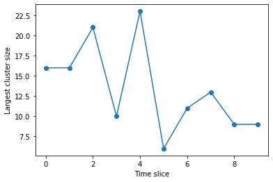
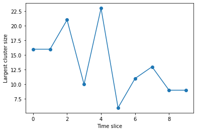
We can also plot the biggest cluster size

plt.plot(range(len(q6clusters)), [max(x) for x in q6clusters], 'o-')
plt.xlabel("Time slice")
plt.ylabel("Largest cluster size")

Text(0, 0.5, 'Largest cluster size')

The final thing to do is to remove the split files after use.

for file in files:
    os.remove(file)

Using ASE

The above example can also done using ASE. The ASE read method needs to be imported.

from ase.io import read

traj = read("traj.light", format="lammps-dump-text", index=":")

In the above function, index=":" tells ase to read the complete trajectory. The individual slices can now be accessed by indexing.

traj[0]

Atoms(symbols='H500', pbc=True, cell=[18.21922, 18.22509, 18.36899], momenta=...)

We can use the same functions as above, but by specifying a different file format.

q6clusters_ase = [calculate_q6_cluster(x, format="ase") for x in traj]

We will plot and compare with the results from before,

plt.plot(range(len(q6clusters_ase)), [max(x) for x in q6clusters_ase], 'o-')
plt.xlabel("Time slice")
plt.ylabel("Largest cluster size")

Text(0, 0.5, 'Largest cluster size')

As expected, the results are identical for both calculations!