Find neighbors of an atom and calculating coordination numbers
In this example, we will read in a configuration from an MD simulation and then calculate the coordination number distribution. This example assumes that you read the basic example.
import pyscal.core as pc
import numpy as np
import matplotlib.pyplot as plt
Read in a file
The first step is setting up a system. We can create atoms and
simulation box using the crystal_structures module. Let us
start by importing the module.
import pyscal.crystal_structures as pcs
atoms, box = pcs.make_crystal('bcc', lattice_constant= 4.00, repetitions=[6,6,6])
The above function creates an bcc crystal of 6x6x6 unit cells with a
lattice constant of 4.00 along with a simulation box that encloses the
particles. We can then create a System and assign the atoms and box
to it.
sys = pc.System()
sys.atoms = atoms
sys.box = box
Calculating neighbors
We start by calculating the neighbors of each atom in the system. There
are two ways to do this, using a cutoff method and using a
voronoi polyhedra method. We will try with both of them. First we
try with cutoff system - which has three sub options. We will check each
of them in detail.
Cutoff method
Cutoff method takes cutoff distance value and finds all atoms within the cutoff distance of the host atom.
sys.find_neighbors(method='cutoff', cutoff=4.1)
Now lets get all the atoms.
atoms = sys.atoms
let us try accessing the coordination number of an atom
atoms[0].coordination
14
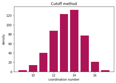
As we would expect for a bcc type lattice, we see that the atom has 14 neighbors (8 in the first shell and 6 in the second). Lets try a more interesting example by reading in a bcc system with thermal vibrations. Thermal vibrations lead to distortion in atomic positions, and hence there will be a distribution of coordination numbers.
sys = pc.System()
sys.read_inputfile('conf.dump')
sys.find_neighbors(method='cutoff', cutoff=3.6)
atoms = sys.atoms
We can loop over all atoms and create a histogram of the results
coord = [atom.coordination for atom in atoms]
Now lets plot and see the results
nos, counts = np.unique(coord, return_counts=True)
plt.bar(nos, counts, color="#AD1457")
plt.ylabel("density")
plt.xlabel("coordination number")
plt.title("Cutoff method")
Adaptive cutoff methods
pyscal also has adaptive cutoff methods implemented. These methods
remove the restriction on having a global cutoff. A distinct cutoff is
selected for each atom during runtime. pyscal uses two distinct
algorithms to do this - sann and adaptive. Please check the
documentation
for a explanation of these algorithms. For the purpose of this example,
we will use the adaptive algorithm.
adaptive algorithm
sys.find_neighbors(method='cutoff', cutoff='adaptive', padding=1.5)
atoms = sys.atoms
coord = [atom.coordination for atom in atoms]
Now let us plot
nos, counts = np.unique(coord, return_counts=True)
plt.bar(nos, counts, color="#AD1457")
plt.ylabel("density")
plt.xlabel("coordination number")
plt.title("Cutoff adaptive method")
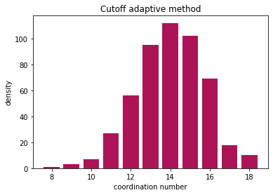
The adaptive method also gives similar results!
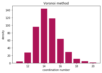
Voronoi method
Voronoi method calculates the voronoi polyhedra of all atoms. Any atom that shares a voronoi face area with the host atom are considered neighbors. Voronoi polyhedra is calculated using the Voro++ code. However, you do not need to install this specifically as it is linked to pyscal.
sys.find_neighbors(method='voronoi')
Once again, let us get all atoms and find their coordination
atoms = sys.atoms
coord = [atom.coordination for atom in atoms]
And visualise the results
nos, counts = np.unique(coord, return_counts=True)
plt.bar(nos, counts, color="#AD1457")
plt.ylabel("density")
plt.xlabel("coordination number")
plt.title("Voronoi method")
Finally..
All methods find the coordination number, and the results are comparable. Cutoff method is very sensitive to the choice of cutoff radius, but Voronoi method can slightly overestimate the neighbors due to thermal vibrations.